Meta-analysis in R

Meta-analysis

Meta-analysis is the quantitative summary of effect sizes extracted from “published” sources. A systematic review doesn’t have to have a meta-analysis (but a meta-analysis needs a systematic review).

What is an effect size?

An effect size is the size of the effect!

The easiest way to think about them is to think of a classic experiment where we compare the effect of an intervention by using a randomised controlled trial.

We can simulate some data from a ten experiments (studies) to show the difference between an intervention and a control group. Let’s imagine we are studying the effect of a restoration intervention on the species richness of beetles.

data <- data.frame(
  study_id = c(1:10,10),
  # Mean species richness in restored and control sites
  mean_restored = c(12, 15, 14, 20, 8, 13, 16, 19, 10, 18, 17),
  mean_control = c(9, 12, 11, 15, 10, 11, 14, 17, 9, 14, 14),
  # Standard deviations for restored and control groups
  sd_restored = c(2.1, 3.0, 2.5, 3.5, 2.0, 2.8, 3.2, 2.9, 2.3, 3.1, 3),
  sd_control = c(2.0, 2.9, 2.6, 3.2, 1.9, 2.5, 2.9, 2.7, 2.1, 2.8, 2.7),
  # Sample sizes for restored and control groups
  n_restored = c(30, 45, 40, 50, 25, 38, 60, 48, 35, 42, 42),
  n_control = c(30, 45, 40, 50, 25, 38, 60, 48, 35, 42, 42)
)

data |> head()

  study_id mean_restored mean_control sd_restored sd_control n_restored
1        1            12            9         2.1        2.0         30
2        2            15           12         3.0        2.9         45
3        3            14           11         2.5        2.6         40
4        4            20           15         3.5        3.2         50
5        5             8           10         2.0        1.9         25
6        6            13           11         2.8        2.5         38
  n_control
1        30
2        45
3        40
4        50
5        25
6        38

Step 1: Calculating the Standardized Mean Difference (SMD)

The standardized mean difference (SMD) between restored and control sites is calculated as follows:

\[\text{SMD} = \frac{\text{mean}_{\text{restored}} - \text{mean}_{\text{control}}}{\text{pooled standard deviation}}\] Where the pooled standard deviation is calculated as:

\[2SD_{\text{pooled}} = \sqrt{\frac{(n_{\text{restored}} - 1) \cdot SD_{\text{restored}}^2 + (n_{\text{control}} - 1) \cdot SD_{\text{control}}^2}{n_{\text{restored}} + n_{\text{control}} - 2}}\]

Let’s calculate this in R:

# Calculate pooled standard deviation and SMD for each study
data$sd_pooled <- with(data, sqrt(((n_restored - 1) * sd_restored^2 + (n_control - 1) * sd_control^2) / (n_restored + n_control - 2)))
data$smd <- with(data, (mean_restored - mean_control) / sd_pooled)

# Calculate variance of the SMD
data$smd_variance <- with(data, ((n_restored + n_control) / (n_restored * n_control)) + (smd^2 / (2 * (n_restored + n_control))))

# View the calculated effect sizes and variances
print(data[c("study_id", "smd", "smd_variance")])

   study_id        smd smd_variance
1         1  1.4629795   0.08450258
2         2  1.0168031   0.05018827
3         3  1.1762445   0.05864719
4         4  1.4910434   0.05111605
5         5 -1.0253040   0.09051248
6         6  0.7535108   0.05636696
7         7  0.6549461   0.03512064
8         8  0.7138306   0.04432059
9         9  0.4540766   0.05861561
10       10  1.3541827   0.05853459
11       10  1.0511767   0.05419626

In ecology we often have small sample sizes, so we use Hedges g to “correct” for small samples. In the R package metafor we can calculate this:

hedges_g_data <- metafor::escalc(measure = "SMD",
                        m1i = mean_restored, sd1i = sd_restored, n1i = n_restored,
                        m2i = mean_control, sd2i = sd_control, n2i = n_control,
                        data = data)

# View the results
hedges_g_data |> 
  select(study_id, yi, vi) |> 
  head()

  study_id      yi     vi 
1        1  1.4440 0.0840 
2        2  1.0081 0.0501 
3        3  1.1649 0.0585 
4        4  1.4796 0.0509 
5        5 -1.0092 0.0902 
6        6  0.7458 0.0563 

Running a meta-analysis

fixed effects vs random effects

In meta-analysis, fixed-effects models assume that all studies estimate the same underlying effect size, with any differences among study results being solely due to sampling error. This model is appropriate when we believe that the effect size is constant across all studies, meaning each study measures exactly the same phenomenon.

In contrast, random-effects models assume that the true effect size varies from study to study due to real differences in study characteristics, such as differences in species, locations, or experimental conditions. Random-effects models treat these variations as random and allow for both within-study sampling error and between-study variability. This is often more realistic in ecology, where conditions across studies are rarely identical.

Accounting for non-independence

Where multiple effects come from a single study (or even from related species!) we need to account for non-independence. We can do this in the meta-analysis model.

ran_eff_model<-
  rma.mv(yi, 
         vi, 
         random = ~ 1 | study_id, 
         data = hedges_g_data)

summary(ran_eff_model)

Multivariate Meta-Analysis Model (k = 11; method: REML)

  logLik  Deviance       AIC       BIC      AICc   
 -9.7272   19.4543   23.4543   24.0595   25.1686   

Variance Components:

            estim    sqrt  nlvls  fixed    factor 
sigma^2    0.4078  0.6386     10     no  study_id 

Test for Heterogeneity:
Q(df = 10) = 61.8318, p-val < .0001

Model Results:

estimate      se    zval    pval   ci.lb   ci.ub      
  0.7940  0.2151  3.6912  0.0002  0.3724  1.2156  *** 

---
Signif. codes:  0 '***' 0.001 '**' 0.01 '*' 0.05 '.' 0.1 ' ' 1

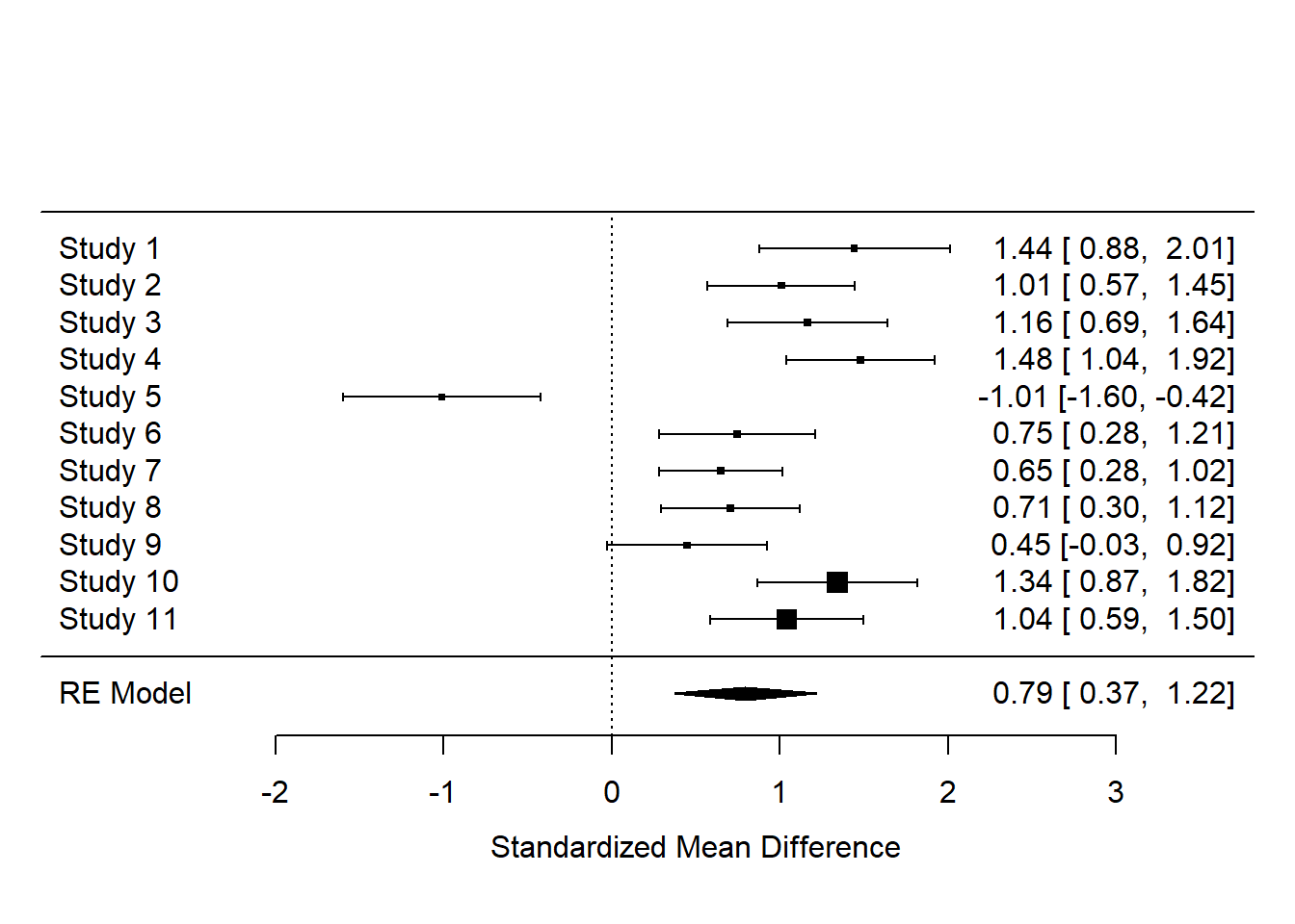
Forest plot

forest(ran_eff_model)

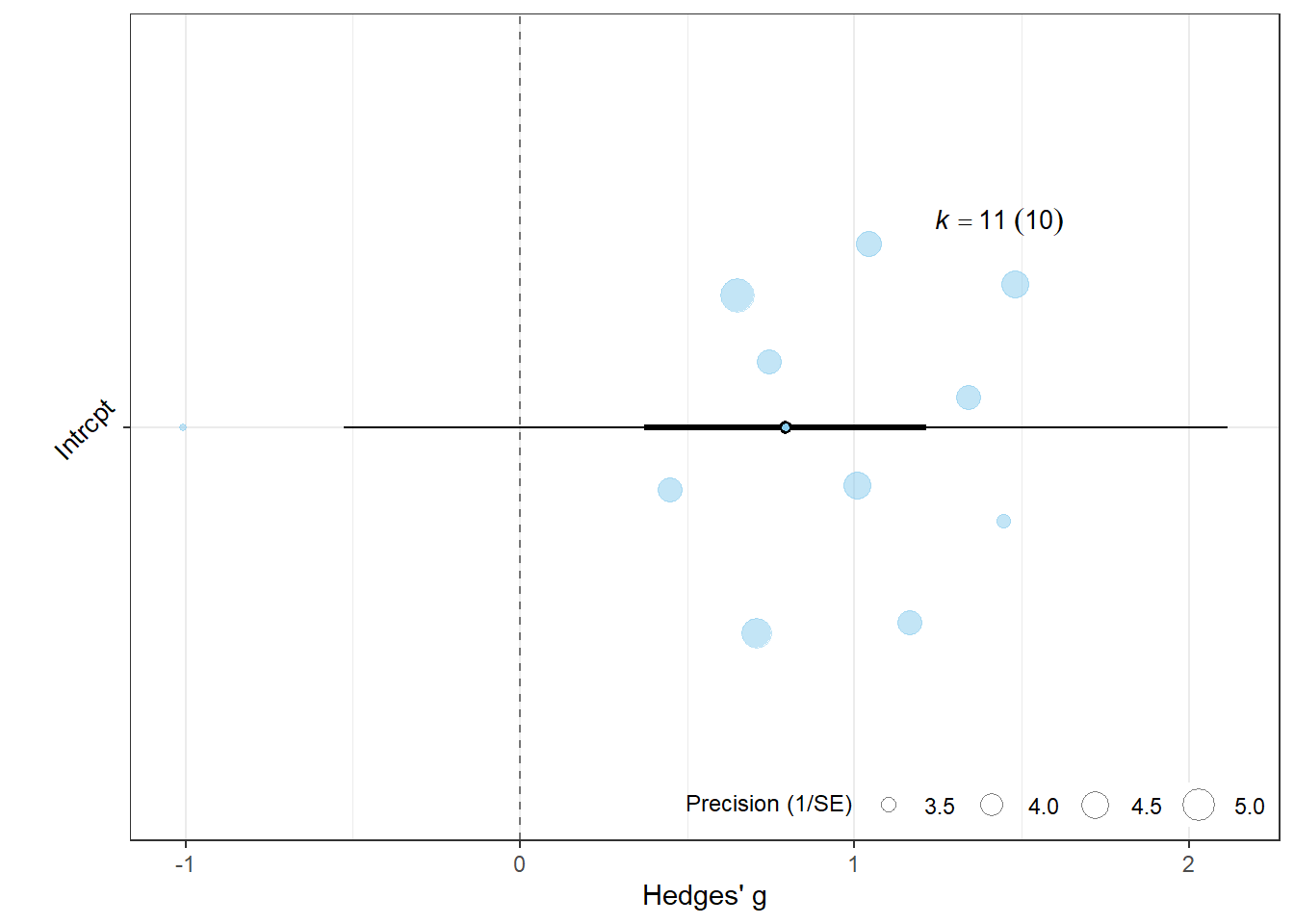
Orchard plots

orchard_plot(ran_eff_model, mod = "1", xlab = "Hedges' g", angle = 45, group="study_id")

Pitfalls with Hedges g

It is very easy to make a mistake in extracting data for calulating the Hedges g. As a “rule of thumb” a Hedges g of greater than 5 should be double/tripple checked.

Here is a link to my Hedges g checker

Cumulative meta-analysis

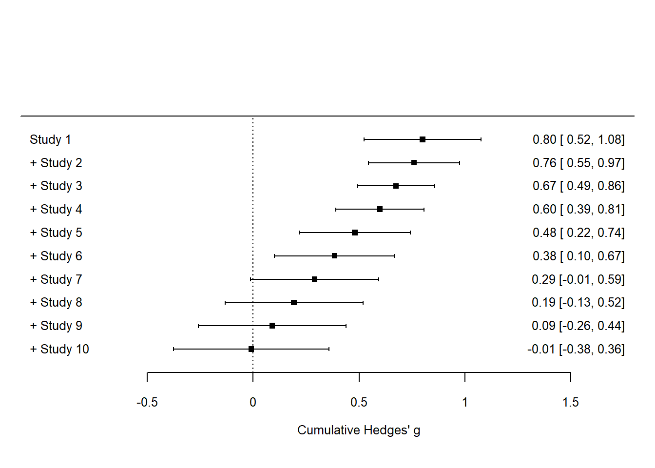
A cumulative meta-analysis examines how the overall effect size estimate changes as each study is added sequentially, usually sorted by publication date. This approach can reveal trends over time, showing whether the effect size has stabilised as more studies are included.

Let’s go through an example of performing a cumulative meta-analysis with the metafor package in R.

Step 1: Create the Dataset

First, we’ll create a dataset with a year variable to sort studies in chronological order for the cumulative analysis.

data <- data.frame(
  study_id = 1:10,
  year = c(2000, 2002, 2004, 2005, 2006, 2008, 2010, 2012, 2015, 2018),  # Publication year
  yi = c(0.8, 0.7, 0.5, 0.3, 0.1, -0.1, -0.3, -0.5, -0.7, -0.9),  # Effect sizes (Hedges' g)
  vi = c(0.02, 0.03, 0.025, 0.04, 0.018, 0.027, 0.035, 0.033, 0.02, 0.03)  # Variances
)

# Sort data by year for cumulative meta-analysis
data <- data[order(data$year), ]

Step 2: Perform Cumulative Meta-Analysis

Now, we can use the cumul() function from metafor to perform a cumulative meta-analysis. This function recalculates the meta-analysis result each time a new study is added.

# Fit an initial random-effects model 
random_effect_model <- rma(yi = yi, vi = vi, data = data, method = "REML")  # Perform cumulative meta-analysis 
cumulative_results <- cumul(random_effect_model, order = data$year)  # View cumulative meta-analysis 
cumulative_results

   estimate     se    zval  pvals   ci.lb  ci.ub        Q     Qp   tau2      I2 
1    0.8000 0.1414  5.6569 0.0000  0.5228 1.0772   0.0000 1.0000 0.0000  0.0000 
2    0.7600 0.1095  6.9378 0.0000  0.5453 0.9747   0.2000 0.6547 0.0000  0.0000 
3    0.6748 0.0938  7.1978 0.0000  0.4911 0.8586   2.0270 0.3629 0.0020  7.4829 
4    0.5986 0.1060  5.6447 0.0000  0.3907 0.8064   4.9607 0.1747 0.0174 38.6738 
5    0.4802 0.1343  3.5758 0.0003  0.2170 0.7434  15.5708 0.0037 0.0642 71.9936 
6    0.3842 0.1449  2.6517 0.0080  0.1002 0.6681  25.8529 0.0001 0.0997 79.8004 
7    0.2904 0.1548  1.8756 0.0607 -0.0131 0.5939  37.8277 0.0000 0.1403 84.2217 
8    0.1927 0.1661  1.1607 0.2458 -0.1327 0.5182  55.7933 0.0000 0.1923 87.7058 
9    0.0898 0.1780  0.5047 0.6138 -0.2590 0.4387  92.8590 0.0000 0.2578 90.8532 
10  -0.0087 0.1871 -0.0462 0.9631 -0.3754 0.3581 123.1155 0.0000 0.3224 92.4608 
        H2 
1   1.0000 
2   1.0000 
3   1.0809 
4   1.6306 
5   3.5706 
6   4.9506 
7   6.3378 
8   8.1339 
9  10.9328 
10 13.2640 

Step 3: Plot the Cumulative Meta-Analysis

You can also visualize the cumulative effect size estimates over time using forest().

# Plot cumulative meta-analysis results 
forest(cumulative_results, xlab = "Cumulative Hedges' g", refline = 0, cex = 0.8)

Interpretation

As you add each study (from the earliest to the most recent), you’ll see how the cumulative estimate of Hedges’ g changes. In ecology, this can highlight if early results were consistent with later studies or if new findings led to significant shifts in the overall effect estimate. This approach provides insight into whether further studies are likely to meaningfully alter the cumulative effect size or if it has stabilised.